The RIGHT(), LEFT(), and MID() formulas are among the most commonly used in Excel. These formulas are commonly used for Data Manipulation, such as trimming or substring a Text from a Cell or from a Constant. Let’s delve deeper with more real-time scenarios.
Syntax :
=LEFT(text,[num_chars])
=RIGHT(text,[num_chars])
=MID(text,start_num,num_chars)
Arguments :
text – It is an optional value that can be either a cell reference or a text constant.
num chars – This parameter must be a number and is optional. This argument instructs the controller to search for the location where the Text should be trimmed. (The initial value is 1)
start_num – This argument, which is required, must contain a number and is used to specify where in the text the text should begin.
RIGHT() / LEFT() /MID() Formula Supported Software products :
- Microsoft Excel
- Google Spreadsheet
- Open Office
- Zoho Excel
Examples :
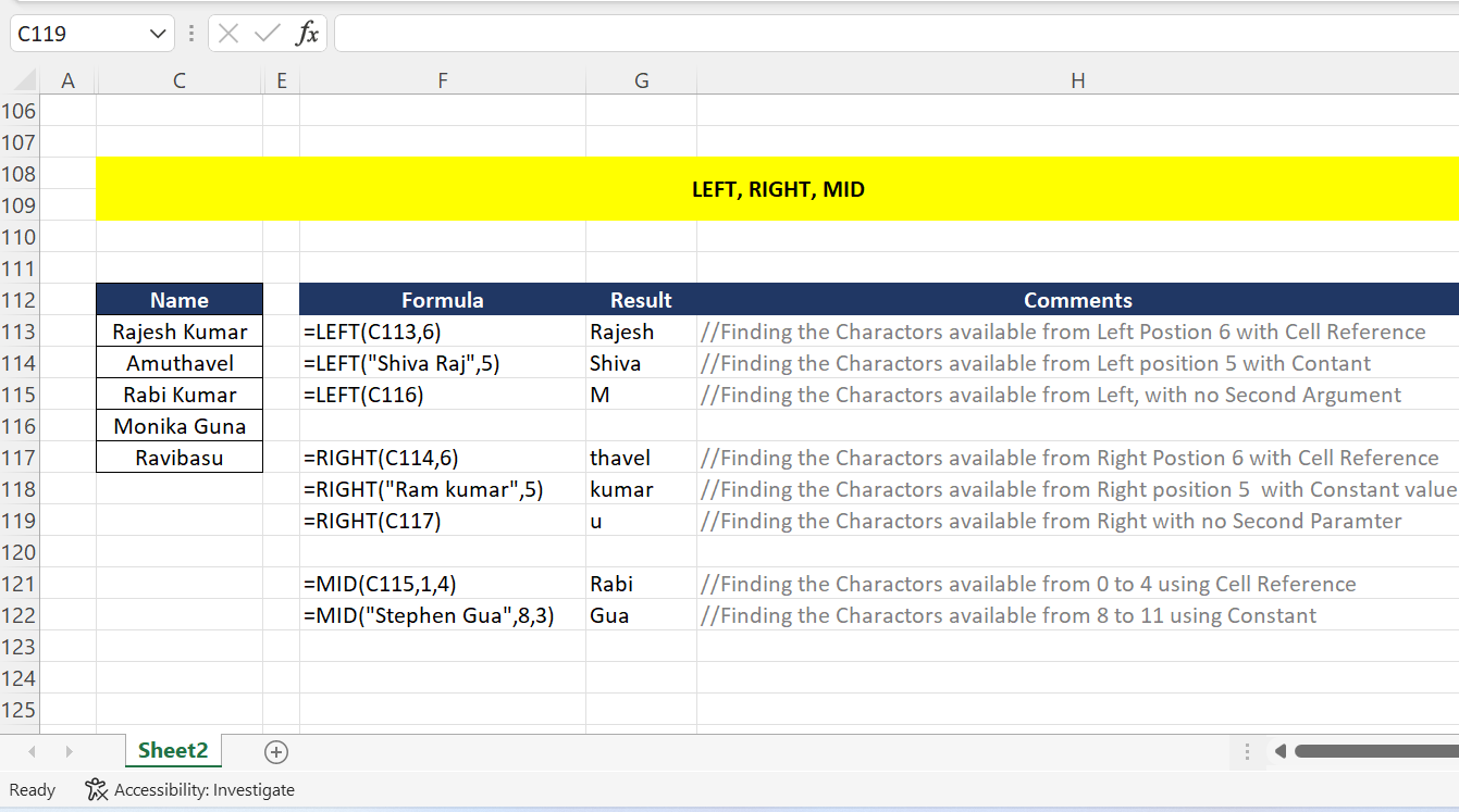
Examples – LEFT() Function :
=LEFT(C113,6) //Rajesh
=LEFT(“Shiva Raj”,5) //Shiva
=LEFT(C116) //M
In the preceding example, we used the LEFT() formula with Cell Reference and Constant as the first parameters. The result will be returned based on the position specified in the second parameter.
For the first two examples, the position value will be calculated from left to right, so the results will be “Rajesh” and “Shiva”. In the third example, there is no position defined; therefore, the controller will consider the default value as 1, and the result will be “M”.
Examples – RIGHT() Function :
=RIGHT(C114,6) //thavel
=RIGHT(“Ram kumar”,5) //kumar
=RIGHT(C117) //u
The RIGHT() formula, which is used to trim content from the right, was used in the instances above. On the first two, the data was trimmed from the right according to the location defined, and as a result, the output printed “thavel” and “kumar.”
Since the second parameter for the third formula was not defined, the system used 1 as the default value and printed “u” as the first character from the right.
Examples – MID() Function :
=MID(C115,1,4) //Rabi
=MID(“Stephen Gua”,8,3) //Gua
In the preceding example, we used the MID() Formula to trim the Content from a Constant or a cell reference. Here, we have used the second argument (start_num) as 1,8 respectively, which means that the system will only look for characters from this. The third parameter was set to 4, 3, which is the number of characters to trim from the starting position. As a result, the final output was “Rabi” and “Gua” respectively.
Points to be noted :
- The Text parameter may be used as a Constant or through Cell Reference.
- Text arguments may contain special characters and any data type.
- If we specify the starting position as 0 or less than that, we used to get an error saying, “Starting Position does not exist.” For MID() Formula, the starting position must be greater than 0.
- Argument – Number of Chars is optional, If we don’t supply the information, the system will use 1 as the default value.

